Imagine the following scenario:

• You possess the position and velocity of a particle at a certain moment.
• You know the net force acting on that particle at that instant.
• However, you lack the equation of motion for the particle.

What steps should you take? The core concept here is numerical computation. By dividing the problem into small time intervals, you can predict the future motion of the object, making approximations during each step to arrive at a solution.

Here’s the plan: I will first analyze a situation where an analytical solution is possible without resorting to numerical methods. Subsequently, I will apply two distinct numerical methods and compare the outcomes. This should be an exciting exploration!

Mass on a Spring

This scenario represents the classic simple harmonic oscillator. Rather than going into all the intricate details, I'll provide a brief overview. You have a mass attached to a spring, resting on a horizontal surface without friction. When the displacement is zero (x = 0 meters), the object remains stationary, facing no forces.

However, once the object is displaced, a restoring force from the spring comes into play. Here’s a diagram—drawing springs is not my favorite task.

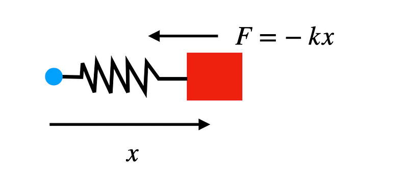
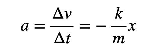
In this one-dimensional scenario (referred to as the x-direction), the only force acting on the mass allows us to express Newton’s Second Law as follows:

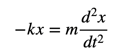
Indeed, this forms a differential equation. We can solve it by making an educated guess for the solution, but it becomes easier to express it as follows:

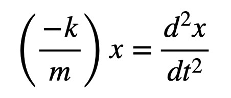
This equation indicates that the function x(t) must be such that taking its second derivative yields the same function multiplied by a constant. Several functions satisfy this condition, but I will opt for sine and cosine. Let's hypothesize this solution and verify if it holds.

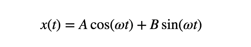
I’ll bypass the intermediate steps here, as my focus is on numerical calculations. If needed, I can create a dedicated post just for solving this equation. However, when I displace the mass to the position x0 and release it with an initial velocity of 0 m/s, I derive the following function.

This represents an analytical solution, allowing me to input any time value to retrieve the mass's position. It's incredible how this works! I can now use this analytical solution to compare various numerical methods. Let’s dive in.

Euler Method

I'll commence with the most straightforward numerical calculation method, which I frequently employ due to its simplicity. Here’s the basic procedure.

First, I start with the initial conditions: I need to know the initial position, velocity, and time. Next, I’ll consider a small time interval (for instance, 0.1 seconds). During this interval, I can compute the object's acceleration using the net force on the mass. Assuming constant acceleration (which it isn't, but it's a reasonable approximation), I can also express acceleration as the change in velocity divided by the time interval.

Let’s say the velocity at the start of this interval is v1, and at the end, it’s v2. I can use the above formula to calculate this final velocity. It is represented as follows:

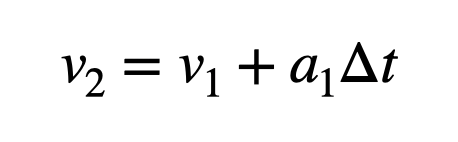
I have not elaborated the expression for acceleration so that this method can be applied to other situations. However, it's crucial to note that the acceleration is calculated based on the position at the beginning of this time interval (hence the subscript 1).

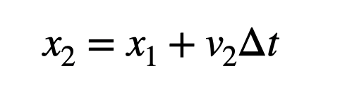
Next, I must update the position of the object during this brief time interval. Again, I will assume the velocity remains constant (which it technically does not). Using the definition of constant velocity:

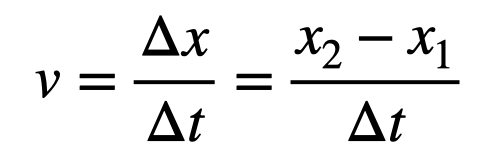
I explicitly illustrate the change in position to clarify when I compute the position at the end of the time interval. I’m also incorporating a little trick here.

Notice the trick? I’m utilizing the velocity at the END of the time interval. Technically, this isn't the pure Euler method since it relies on the velocity at the end of the interval. This approach is actually referred to as the Euler-Cromer method.

After updating the position, we can proceed to the next time interval and repeat the process.

Here’s some basic Python code illustrating how this would function (using VPython Glowscript). A vital aspect of numerical calculation is that you need specific numerical values (mass, spring constant, initial position) for computations. Here’s the basic code (you can find the actual code here).

t = 0

dt = 0.1

x = 0.05

k = 10

m = 1

v = 0

while t < 3:

a = -k * x / m

v = v + a * dt

x = x + v * dt

fe.plot(t, x)

t = t + dt

One important note regarding this code: observe the line below.

v = v + a * dt

The equal sign here does not signify algebraic equality. Instead, it conveys that we are assigning the value obtained from the right side to the left. In Python, this line indicates to take the current velocity (whatever value is assigned to that variable) and add the product of “a” and “dt”, then assign this resultant value to “v”. In this sense, this aligns with the velocity update in the Euler method.

Now, let’s examine the comparison between the Euler method and the analytical computation. Here’s a plot showcasing results from the Euler method with a time step of 0.1 seconds alongside another calculation at 0.01 seconds.

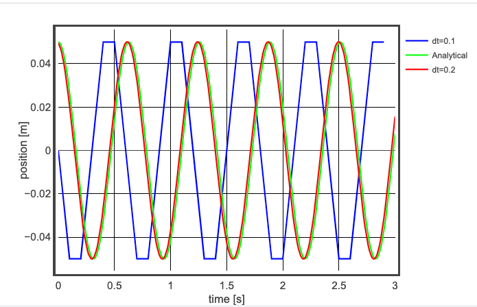
Not too shabby! Even with a larger time step of 0.1 seconds, the Euler method performs reasonably well. While it may not yield the exact position, the oscillation period closely resembles the analytical solution, and the amplitude remains relatively stable. Quite impressive!

By reducing the time interval to 0.01 seconds, the difference between the Euler method and the analytical solution becomes nearly imperceptible. This is why the Euler method is advantageous; it's often accurate and very easy to use, making it ideal for students.

Euler-Richardson (Runge-Kutta-2) Method

This method can be referred to as Euler-Richardson or Runge-Kutta (second order), but perhaps "mid-step method" is a more fitting label. To grasp this method, let’s consider the velocity-time graph for the mass on the spring.

Assuming I apply the Euler method to determine the velocity after a certain time interval, I need the acceleration at that point (which corresponds to the slope of the velocity graph), and it might appear as follows. Yes, my time interval is rather large.

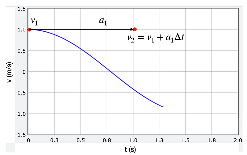
The black arrow signifies the slope at point 1. However, since acceleration is not constant, the projected value for v2 diverges from the theoretical value (as seen in the graph).

The Euler-Richardson method employs a similar approach to determine the new velocity. Instead of using the acceleration (slope) at point 1, it utilizes the slope at the midpoint between times 1 and 2. Observe the difference below.

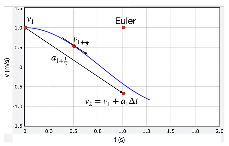
I included the point for the Euler method for comparison purposes. Remember, the acceleration (the slope of this curve) can be derived from the spring force, which is known and depends on position x. However, this introduces a new challenge: how can I ascertain the position at the half-step (x-1/2) if I don't yet know the position at the end of the time interval?

The solution lies in utilizing the basic Euler method with a half-time interval to find the position and velocity at this midpoint.

In this case, I primarily need the midpoint position since the spring's force relies solely on position. If air resistance were involved, I would also require the midpoint velocity to update the position for the full time interval.

Once I have the midpoint position, I can compute the midpoint acceleration.

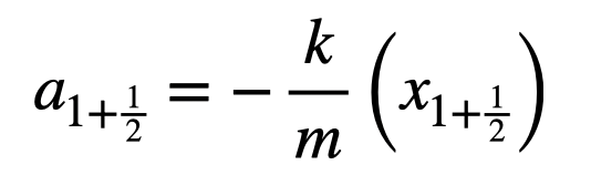
Calculating v2 and x2 mirrors the Euler method but utilizes this midpoint acceleration.

And that’s it!

Now, let’s translate this into Python code. It would look something like this:

while t < 3:

a = -k * x / m

vm = v + a * dt / 2

xm = x + v * dt / 2

am = -k * xm / m

v = v + am * dt

x = x + vm * dt

fe.plot(t, x)

t = t + dt

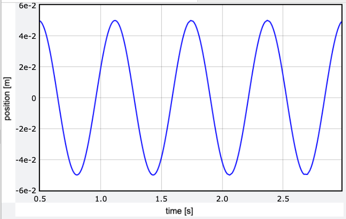
Here’s the actual code, and this is what the output resembles for a significantly large time interval.

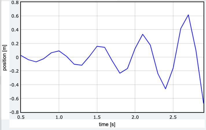
That’s quite poor. Honestly, I’m unsure why the basic Euler method performs better for larger time intervals, but here we are. When I reduce the time interval to 0.01 seconds, the results look promising.

Nonetheless, I feel like something may have gone awry.

Comparing Euler and Euler-Richardson

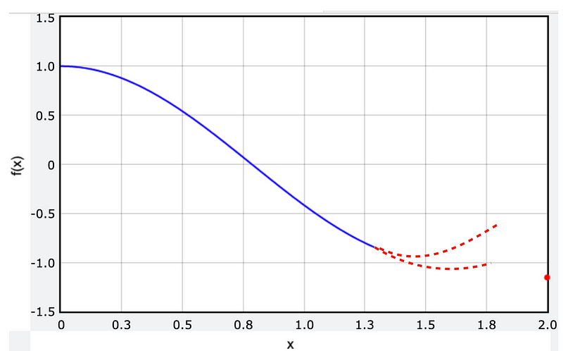
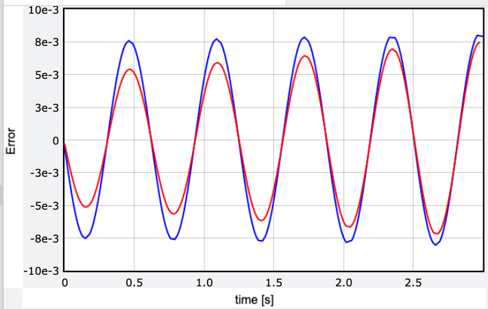
Certainly, I could simply plot the oscillating mass using the two different methods for comparison. However, if the deviation is minimal, it may not be easily noticeable. Instead, I’ll calculate the mass's position at various time intervals and plot the deviation of each method from the analytical solution. This is how it looks with a significantly large time interval of 0.1 seconds. The red curve represents the Euler-Richardson method, while the blue curve depicts the basic Euler method (technically the Euler-Cromer).

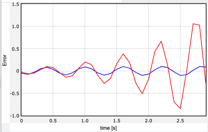
In this case, Euler exhibits a smaller deviation. But what happens with a time interval of 0.01 seconds?

Now, the Euler-Richardson method outperforms.

There are likely more effective ways to assess the error in numerical calculations, but I’ll pause here since I don't feel entirely confident in my Euler-Richardson method.

What I am certain about is that the Euler-Cromer method is generally reliable for most scenarios. When it falters, reducing the time interval is a simple fix. Sure, it may seem primitive, but it does the job.