An Integral Perspective on Geometric Series

How does the geometric series link to singularities and generating functions? This exploration is part of "Infinity: The Math Odyssey," where I delve into the early mathematical approaches to understanding infinity through series—specifically, the process of infinitely summing quantities that converge to a finite number.

The telescoping series has evolved into a cornerstone of calculus, connecting to the fundamental theorem of calculus. Meanwhile, the geometric series has proven to be an ideal framework for investigating singularities. This recursive nature directly relates to the concept of infinity and singularities.

Motivation: The geometric series ties closely to two areas I plan to explore in future writings: singularity and generating functions. Hence, it is essential to articulate this narrative as well.

Introduction to Geometric Series

What exactly constitutes a number, such as 2? It symbolizes a quantity—specifically, the concept of repeating unity twice. Suppose we define 2 using a series, particularly through infinite summation. This concept resembles Zeno's paradox, where we continuously halve the number 2:

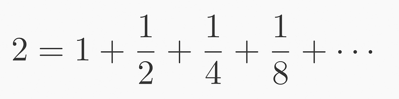
We begin by halving 2 to get 1, then halve the remainder to yield 1/2, continuing until we sum infinitesimal values approaching zero. While we know the end result is 2, it is formed from fractional components.

This series is geometric because each subsequent term's size is a constant fraction of the previous term, with the ratio for 2 being 0.5 or 1/2.

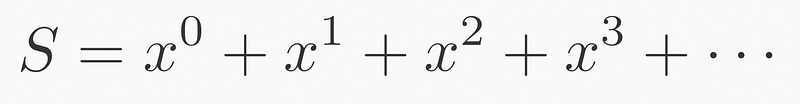
This principle can be generalized for any ratio, not limited to 1/2, by using its power:

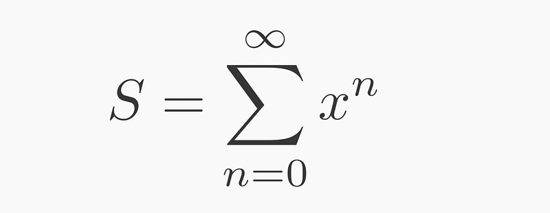
Expressing this series in sigma notation yields:

To derive a formula for this series, we can factor out from ( x^1(1+x+x^2+ldots) ):

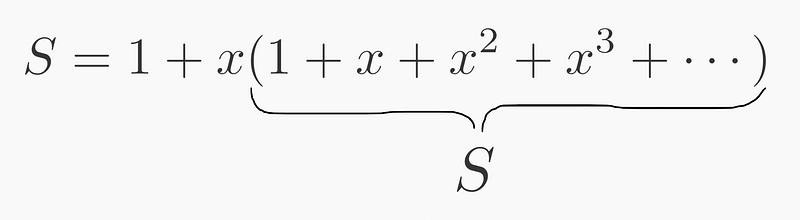
Notice that this recursive behavior allows us to isolate ( S ) on the right, thus enabling further factorization:

Through straightforward algebraic manipulation, we arrive at:

Conclusion

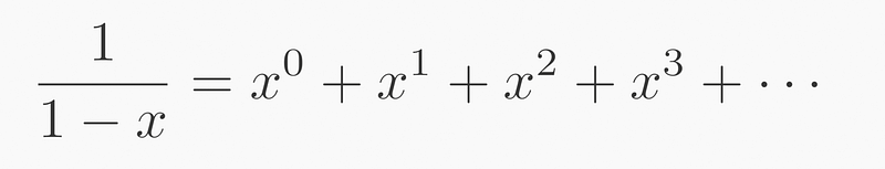
In this exercise, we demonstrated that a pole (singularity) at ( x=1 ) in ( frac{1}{1-x} ) corresponds to the infinite sum of ( x^n ).

Understanding Singularity

I've frequently referred to poles, which denote locations where a function approaches "infinity" or, more accurately, where it is undefined. For ( frac{1}{1-x} ), this occurs at ( x=1 ). Poles can also be viewed as the roots of the denominator.

There exist various types of singularities in mathematics, but I will focus on poles, which are a form of analytical singularity—an aspect we can study and analyze. Analytical functions can be represented as polynomials via Taylor series, and we extend this idea to encompass functions that are not strictly analytical—leading us to meromorphic functions.

Meromorphic functions consist of both a numerator and denominator that are analytic. We no longer need to avoid issues of division by zero; instead, we will focus on the locations and circumstances of such divisions. Ironically, while we previously sought to avoid ( frac{1}{0} ), this expression will become a primary focus of our study.

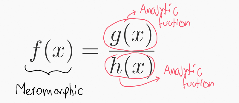
The poles are the roots of the polynomial ( h(x) ), defined as the values where ( h(x)=0 ), which we will refer to as the singularities of the function ( f(x) ).

Poles: In real analysis, we deemed these points undefined, but in complex analysis, the notion of 'undefined' is supplanted by information regarding residues.

Poles are singularities that possess a residue, according to Cauchy's residue theorem. However, our current discussion is about demonstrating that poles (a type of singularity) are equivalent to sequences.

Instead of consistently using "pole," I may refer to it as "singularity," although remember there are various types. This particular type allows for analysis, meaning:

A singularity can be expressed as a sequence (with different bases, in this case, ( x^n ) or what I refer to as Taylor series bases).

Spoiler: What if we attempt to sum ( 1+2+4+8+16+ldots )? This equivalence suggests it equals -1. Previously, we regarded ( 1+2+4+8+ldots ) as diverging to infinity; now we assert it equals -1. Why? Perhaps this will be clearer in a future explanation (hint: p-adic numbers and transfinites).

Most mathematicians (if not all) will initially declare this assertion (that ( 1+2+4+8+ldots = -1 )) to be erroneous. This was the consensus before the advent of p-adic numbers, which will clarify this notion in the future. This also relates to the famous series ( 1+2+3+4+5+ldots = -frac{1}{12} ), where the answer derives from the concept of analytic continuation, further elucidated by p-adic numbers.

Generating Functions

There are two methods to construct an "analytic" sequence:

1. Absolute indexing
2. Recursive indexing

As evidenced in the Fibonacci sequence, a sequence can be derived from previous terms (adding the last two), but it can also be determined through a formula that does not rely on the last terms of the sequence (e.g., Binet's formula). For instance, to find the 57th term in the Fibonacci sequence, knowing the 55th and 56th terms suffices, but to find it directly, one can simply exponentiate the poles to the 57th power.

• Absolute indexing ? powering the poles.
• Recursive indexing ? functional form of the poles (rearranging the denominator).

A singularity like ( frac{1}{1-x} ) represents a sequence of [1,1,1,1,…]. The coefficients of the Taylor series reflect this sequence. We now occupy a novel space, where ( x^n ) denotes the bases and its coefficients represent the values.

To introduce the dot product concept, we can express it as follows:

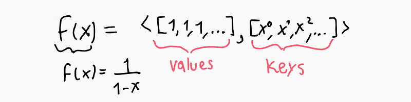
We have two vectors: one filled with ones and the other containing ( x^n ). The dot product is obtained by multiplying one vector by the other and summing the results, denoted as ( langle text{vector1}, text{vector2} rangle ). This interpretation will facilitate the application of this concept to both discrete sequences and continuous functions in the future.

Our sequence can be recursively described as equivalent to its prior value:

This indicates that in generating functions, the function equals itself lagged by one step:

It's worth noting that we use an uppercase 'F' to denote the generating function. We will operate within two distinct realms: one dedicated to the coefficients of sequences and the other for generating functions.

If we seek the function that adheres to the recursive rule described above, we discover it closely resembles ( frac{1}{1-x} ), merely missing an element (to be explained later). Why is it zero instead of one?

What does lagging mean when we multiply by ‘x’? If we consider the coefficient of a Taylor series as the sequence of interest, such as [1,2,3,4,5,…], how do we derive the same sequence shifted one position to the right? [0,1,2,3,4,5,…].

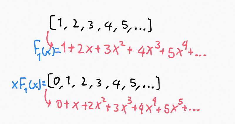
By multiplying by 'x', we effectively shift the sequence in relation to its power ( x^n ).

Revisiting Concepts

I find it challenging to connect certain concepts to what I've previously articulated, so I will isolate them for clarity.

Geometric Transformation: Grasping the concept of infinity can be complex; here, "geometric" carries a meaning distinct from "geometric series." In this context, I refer to rotations (a type of geometric transformation). They are indeed interconnected, but let’s consider an example.

Imagine an infinite line of people. Can you point out where the end of the line is?

If it extends infinitely, you might think it impossible, right?

In reality, you can, and this phenomenon is termed the vanishing point (as seen in photography).

If we apply a rotation and alter our perspective, regardless of how vast (or infinite) the line may be, one can discern its endpoint at the vanishing point.

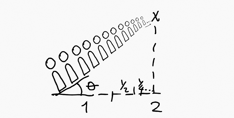
The sequence of projected distances when viewed from an angle does not conform to a geometric sequence; however, the notion remains similar. "Infinity" can be projected onto finite numbers. This idea is further explored in the context of Möbius transformations and the Riemann sphere.

I pose the question again: how can we indicate the end of an infinitely long row when viewed from a rotated perspective?

In a prior narrative, I suggested a thought experiment: what if there were no finite numbers, only infinities? This section aims to reinforce that intuition.

Recursivity vs. Singularity vs. Time Spread Sequence I previously mentioned two methods of expressing a sequence and will now introduce a third. Let’s denote our sequence as twice the last term minus three times the term before that.

Recursive Formulation This follows the recursive rules:

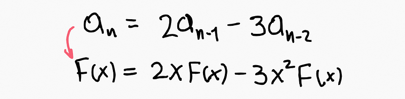
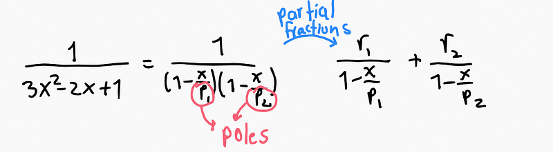
Singularity Formulation When we apply the recursive rules to derive the generating function as a fraction (with poles/singularities playing a key role):

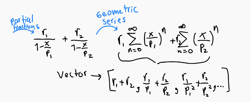
Time Spread Sequence If we reverse the singularities back to their equivalent sequences, we generate a series of infinite numbers, akin to ( 1+2+3+4+ldots ) or any other infinite series.

Convolution: What Does [1,1,1,1,…]*[1,1,1,1,…] Mean? We can multiply finite sequences within a polynomial function, but how do we handle infinite sequences like series? What results from multiplying [1,1,1,1,…]*[1,1,1,1,…]?

We know that [1,1,1,…] corresponds to the generating function ( frac{1}{1-x} ). Thus, multiplying it by itself gives us ( frac{1}{(1-x)^2} ). Now, to discern which values belong to its sequence, consider the “Time Spread Sequence.”

It turns out that multiplying functions equates to applying convolution across their coefficient space.

Spoiler: This concept bears similarities to Laplace and Fourier transforms (which I will discuss in future writings).

In these transforms, multiplication of functions is analogous to applying convolution in another space. The inverse holds true: applying convolution to functions corresponds to multiplying after the Laplace/Fourier transformation.

To multiply the infinite sequence [1,1,1,1,…]*[1,1,1,1,…], we can also express it as ( (1+x+x^2+x^3+ldots)*(1+x+x^2+x^3+ldots) ). By performing the multiplication term by term, one can observe the emerging pattern:

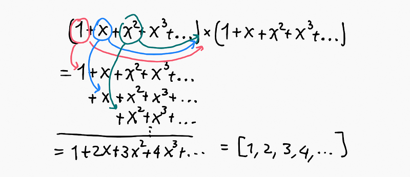
The multiplication of these two functions (or the convolution of their coefficient sequences) results in [1,2,3,4,…]. This becomes clearer when recognizing that each ( x^n ) represents a sequence lagged by ( n ). Thus, each term is a lag, and we sum their results.

I've introduced the concept of evolution here, which may also assist: Demystifying Pascal’s Triangle. In that discussion, we multiplied by ( (1+x) ); here, we multiply by ( (1+x+x^2+ldots) ).

Conclusion

We are focused on studying sequences here. Utilizing the Geometric Series formula, we understand that a sequence [1,1,1,1,…] can be represented as ( frac{1}{1-x} ), which features a pole at ( x=1 ). This has further implications: any sequence can be expressed as a Taylor series, which is a polynomial function, and subsequently as a recursive sequence or pole-sequence.

The degree of the polynomial in the denominator of the generating function—equivalent to the number of poles—also reflects the count of recursive rules or the degree of the Taylor series polynomial.

Consequently, each sequence (time spread) can be articulated as a collection of recursive rules, as well as the summation of its poles raised to ( n ). This relationship stems from connecting the singularity ( frac{1}{1-x} ) with geometric series and sequences through generating functions.

Warnings

Formally, a series possesses a convergence zone and a divergence zone. I may elaborate later on why I regard these as identity connections. The primary reason pertains to p-adic numbers. While in reality, the summation ( 1+2+4+8+ldots ) appears counterintuitive, in mathematics, it is entirely valid. In my view, this holds true in reality as well, provided we adopt a different perspective (as I attempted to illustrate in the section on geometric transformations). The divergence zone represents the analytic extension of the series' convergence zone.

Spoiler: Why does the generating function have a numerator of 0 instead of 1? The missing 1 stems from a delta Dirac input. The generating function operates as a system (input-output); when there is no input, it results in a zero numerator. If it begins with 1, this implies a delta Dirac as input, thus yielding the 1 in the numerator.