Chapter 1: Introduction to the Anomalous Magnetic Moment

In the previous discussion, we explored the interaction of an electron with a photon, aiming to investigate the electron g-factor. We analyzed the probability amplitude associated with this interaction and sought to align it with the g parameter from our foundational equation.

We concluded our earlier analysis by calculating the amplitude at the 'tree level,' which refers to calculations that do not incorporate loop processes. However, to refine our estimation of g, we must include diagrams featuring loops. Loops represent closed segments in these diagrams that provide a 'free' level of momentum available for integration. By summing the probability amplitudes of these loop diagrams, we can achieve a correction to our g-factor. Generally, the amplitude we focus on is the aggregate of all potential loop diagrams resulting from an electron scattering off a photon.

Chapter 2: Examining Loop Diagrams

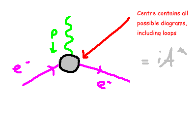
In the preceding diagram, we identify three degrees of freedom relevant to our analysis: the momentum of the photon, the incoming electron, and the outgoing electron. These components interact at the vertex, where potential loop diagrams that could modify our g-factor are also situated. We will delve into two specific examples in the following section.

Now, the critical question arises: how do we perform this calculation? A viable starting point is to formulate the most 'general' expression for this number. As noted in Schwartz's textbook on quantum field theory, the most comprehensive form can be represented as a linear combination of the momentum vectors. For instance, in the equation below, the incoming and outgoing electrons are depicted by the vectors u, while the middle term serves as a general linear combination of factors included in this probability.

Schwartz outlines various arguments that enable us to eliminate certain components from this expression. A fundamental starting point is the principle of momentum conservation; since p=q_2 – q_1, we can directly eliminate p from our expression. Typically, the functions f¹, f², and others can be intricate functions of the three external momenta, and being scalars, they must rely on real numbers rather than vectors.

Due to a reason I won't elaborate on here, we find that these functions can only depend on p² / m², which is the momentum of the photon divided by the mass of the electron. This restriction arises because the momenta of the electrons comply with the Dirac equation and through dimensional analysis. In quantum field theory, momentum is measured in mass units, necessitating division by the electron mass to ensure our function argument is dimensionless.

Section 2.1: The Role of the Ward Identity

We can further refine our amplitude expression using the Ward identity, which asserts that contracting the scattering amplitude with the momentum of an incoming photon should yield zero. This identity simplifies our expression so that our final amplitude relies solely on f¹ and f².

The two terms in this equation are referred to as form functions. The second term modifies the value of g, as it includes a component representing the magnetic moment in momentum space. The correction, in this instance, is represented by F². When dealing with relatively low momentum, the value of p² becomes negligible compared to the electron's mass, resulting in our correction being defined as:

Section 2.2: Analyzing the One Loop Diagram

To ascertain the form factors, we must evaluate the amplitude related to a loop diagram. Constructing such a diagram requires maintaining the same three external legs while incorporating a loop. In the image below, I present two such diagrams. Notably, the first diagram does not contribute to the correction of the magnetic moment, while the second one does.

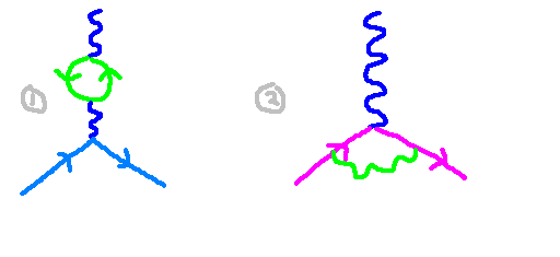
In the subsequent section, I will explain how we compute this diagram and the insights we can derive from it!