Creating Custom Random Number Distributions with Python
Written on
Chapter 1: Introduction to Custom Probability Distributions
In this guide, we will explore how to sample random numbers from various probability distributions using straightforward Python code.
Creating Your Own Probability Distribution
Imagine having the ability to design your own probability distribution. The good news is that you are not limited to the conventional distributions that are commonly used. With the right approach, you can easily create a distribution that suits your specific needs.
To begin, we need to adhere to a few fundamental principles when defining a probability distribution ( p(x) ):
- ( p(x) geq 0 ): This means that ( p(x) ) must be non-negative for all values of ( x ) (where ( x ) is a real number). Negative probabilities are not valid.
- The integral of ( p(x) ) across all possible values of ( x ) must equal one. For discrete distributions, the sum of all ( p(x) ) must also equal one, mathematically expressed as ( sum p(x) = 1 ).
To create a valid probability distribution, we can first define an "un-normalized" distribution ( g(x) ) based on our chosen rules (for instance, ( g(x) = x^2 )), ensuring it meets the first condition. We then normalize it by dividing by the total of its values, resulting in ( p(x) = frac{g(x)}{sum g(x)} ). This normalization guarantees that ( sum p(x) = 1 ).
Let’s experiment with a simple distribution defined by ( g(x) = (x-x_0)^2 ), where ( x_0 ) is a parameter that shifts the parabola to the right. We will assume ( g(x) ) is defined over an interval ([a, b]) and is zero outside this range.
The process is as follows: first, we create an array ( X ) spanning from ( a ) to ( b ), ideally with equal spacing. Next, we compute ( p(X) = frac{g(X)}{sum g(X)} ) and denote this array as ( P ). We then calculate the cumulative sum of ( P ), which we will call ( C ).
At each point in the array ( X ), ( C ) accumulates values, ultimately reaching a maximum of 1 due to the normalization. The next step is to simulate a random number from a uniform distribution, represented as:
( U sim text{Uniform}(0,1) )
We then multiply ( U ) by the final value of ( C ), referred to as ( text{max}(C) ). Alternatively, we can use the last value in ( C ), ( C[-1] ), which also represents ( text{max}(C) ). The goal is to evaluate whether ( U cdot text{max}(C) > C ). This yields a logical array that indicates True (1) or False (0) for each position in ( C ).
For instance, if ( C ) has five values, the resulting logical array from this comparison might look like this:
[ [text{True}, text{True}, text{False}, text{False}, text{True}] equiv [1, 1, 0, 0, 1] ]
By summing the logical array, we determine the index from which we will sample a value from ( X ). This process works because each sampling of ( U ) generates a different index based on the distribution of ( P ).
To illustrate this in Python, the following code demonstrates how to generate random numbers according to an arbitrary probability distribution defined by the user:
# Arbitrary probability distribution
# Generates random numbers according to an arbitrary probability distribution
# p(x) defined by the user on a domain [a,b]
# Author: Oscar A. Nieves
# Last updated: July 30, 2021
import matplotlib.pyplot as plt
import numpy as np
import math as mt
plt.close('all')
# Inputs
a = 10
b = 25
x0 = (a+b)/2
samples = 1000
X = np.linspace(a,b,1001)
# Define p(x)
def g(x_var):
return (x_var - x0)**2
P0 = g(X) # Unnormalized probabilities
# Normalize p(x)
Psum = sum(P0)
P = P0/Psum
# Cumulative sum p(x)
C = np.cumsum(P)
# Compute random numbers
R = np.linspace(a,b,samples)
for n in range(samples):
index0 = mt.ceil(sum(sum(C[-1]*np.random.rand(1,1) > C)))
R[n] = X[index0]
# Generate histogram
bins = 50
plt.subplot(1,2,1)
plt.plot(X,P,color='black')
plt.xlim([a,b])
plt.xlabel('X', fontsize=16)
plt.ylabel('p(x)', fontsize=16)
plt.subplot(1,2,2)
plt.hist(R,bins)
plt.xlim([a,b])
plt.xlabel('R', fontsize=16)
plt.ylabel('frequency', fontsize=16)
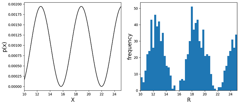
Running this code produces the following plots:
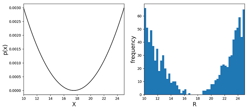
The left side displays the normalized probability distribution ( p(x) ) (or ( P )), while the right showcases a histogram of the randomly sampled numbers ( R ). Here, we generate 1,000 independent samples for ( R ) within a loop. Notably, you can select any function ( g(x) ) that meets the criteria.
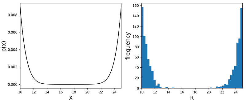
For instance, if we opt for ( g(x) = (x-x_0)^3 ), the output would appear significantly wider around the center:
And that’s it! You now have the knowledge to create any random number distribution you desire. Enjoy experimenting!